The China Syndrome: Autor, Dorn and Hanson (2013), replicated and extended to 2024
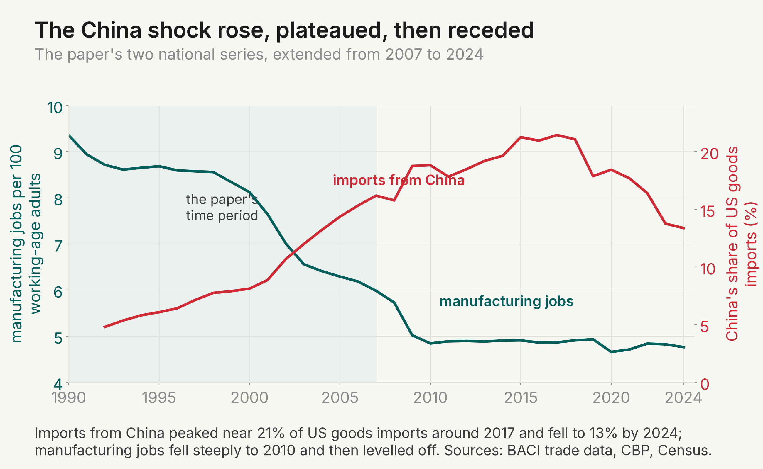
Between 1990 and 2007, China's share of US goods imports rose from under 5 to over 16 percent. Autor, Dorn and Hanson split the country into 722 local labour markets and asked what the surge did to the places making the same goods, using other rich countries' imports from China to strip out anything driven by US demand. The more exposed a place was, the more manufacturing jobs it lost: about 0.6 percentage points for every $1,000 of import growth per worker.
The paper's main claims
- A $1,000 per worker rise in decadal import exposure cuts manufacturing employment per working-age adult by 0.596 percentage points.
- That explains about one quarter of the US manufacturing decline over 1990–2007.
- It also raises unemployment by 0.221 points and non-participation by 0.553 points.
- Average weekly wages fall by 0.759 log points.
- Transfer payments rise by about $58 per capita.
What we got when we re-ran it
We re-ran the authors' published archive and scored 0.80: 19 of 25 scored claims matched (4 of 5 headline claims and 15 of 20 supporting claims; the rest partial, not attempted, or out of scope rather than contradicted). A clean pass. Italicised rows are ours; every cell matches at published precision.
Table 3. Imports from China and Change of Manufacturing Employment in CZs, 1990–2007: 2SLS Estimates
Dependent variable: 10 × annual change in manufacturing emp/working-age pop (in % pts)
Panel I. 1990–2007 stacked first differences
| (1) | (2) | (3) | (4) | (5) | (6) | |
|---|---|---|---|---|---|---|
| (Δ imports from China to US)/worker | −0.746*** | −0.610*** | −0.538*** | −0.508*** | −0.562*** | −0.596*** |
| (0.068) | (0.094) | (0.091) | (0.081) | (0.096) | (0.099) | |
| this replication | −0.746 | −0.610 | −0.538 | −0.508 | −0.562 | −0.596 |
| (0.068) | (0.094) | (0.091) | (0.081) | (0.096) | (0.099) | |
| Percentage of employment in manufacturing₋₁ | −0.035 | −0.052*** | −0.061*** | −0.056*** | −0.040*** | |
| (0.022) | (0.020) | (0.017) | (0.016) | (0.013) | ||
| this replication | −0.035 | −0.052 | −0.061 | −0.056 | −0.040 | |
| (0.022) | (0.020) | (0.017) | (0.016) | (0.013) | ||
| Percentage of college-educated population₋₁ | −0.008 | 0.013 | ||||
| (0.016) | (0.012) | |||||
| this replication | −0.008 | 0.013 | ||||
| (0.016) | (0.012) | |||||
| Percentage of foreign-born population₋₁ | −0.007 | 0.030*** | ||||
| (0.008) | (0.011) | |||||
| this replication | −0.007 | 0.030 | ||||
| (0.008) | (0.011) | |||||
| Percentage of employment among women₋₁ | −0.054** | −0.006 | ||||
| (0.025) | (0.024) | |||||
| this replication | −0.054 | −0.006 | ||||
| (0.025) | (0.024) | |||||
| Percentage of employment in routine occupations₋₁ | −0.230*** | −0.245*** | ||||
| (0.063) | (0.064) | |||||
| this replication | −0.230 | −0.245 | ||||
| (0.063) | (0.064) | |||||
| Average offshorability index of occupations₋₁ | 0.244 | −0.059 | ||||
| (0.252) | (0.237) | |||||
| this replication | 0.244 | −0.059 | ||||
| (0.252) | (0.237) | |||||
| Census division dummies | No | No | Yes | Yes | Yes | Yes |
Panel II. 2SLS first stage estimates
| (1) | (2) | (3) | (4) | (5) | (6) | |
|---|---|---|---|---|---|---|
| (Δ imports from China to OTH)/worker | 0.792*** | 0.664*** | 0.652*** | 0.635*** | 0.638*** | 0.631*** |
| (0.079) | (0.086) | (0.090) | (0.090) | (0.087) | (0.087) | |
| this replication | 0.792 | 0.664 | 0.652 | 0.635 | 0.638 | 0.631 |
| (0.079) | (0.086) | (0.090) | (0.090) | (0.087) | (0.087) | |
| R² | 0.54 | 0.57 | 0.58 | 0.58 | 0.58 | 0.58 |
| this replication | 0.54 | 0.57 | 0.58 | 0.58 | 0.58 | 0.58 |
Notes: N = 1,444 (722 commuting zones × 2 time periods). All regressions include a constant and a dummy for the 2000–2007 period. First stage estimates in panel II also include the control variables that are indicated in the corresponding columns of panel I. Robust standard errors in parentheses are clustered on state. Models are weighted by start of period CZ share of national population. *** Significant at the 1 percent level. ** Significant at the 5 percent level. * Significant at the 10 percent level. Replication: italicised rows are our re-execution of the authors' archive; every cell in both panels matches the published value at published precision (verification verdict C2). Our replication output prints coefficients and standard errors but no significance stars, so the stars shown are the paper's.
The paper's coefficient, period by period:
| 1990–2000 | 2000–2007 | 1990–2007 stacked | |
|---|---|---|---|
| Published | −0.89*** (0.18) | −0.72*** (0.06) | −0.75*** (0.07) |
| This replication | −0.888 (0.181) | −0.718 (0.064) | −0.746 (0.068) |
The same analysis on today's data
We carried the design forward to 2024: trade flows from CEPII BACI, exposure rebuilt with the paper's formulas, outcomes from public sources, specification frozen at Table 3 column 6. The model:
with the change in a zone's manufacturing employment share and Chinese import growth per worker, apportioned by industry mix and instrumented with the same measure built from other rich countries' imports. The effect is fully alive in 2007–2012 at −0.417, on years the authors never saw, fades to zero in 2012–2019, and flips slightly positive in 2019–2024 as the shock itself receded.
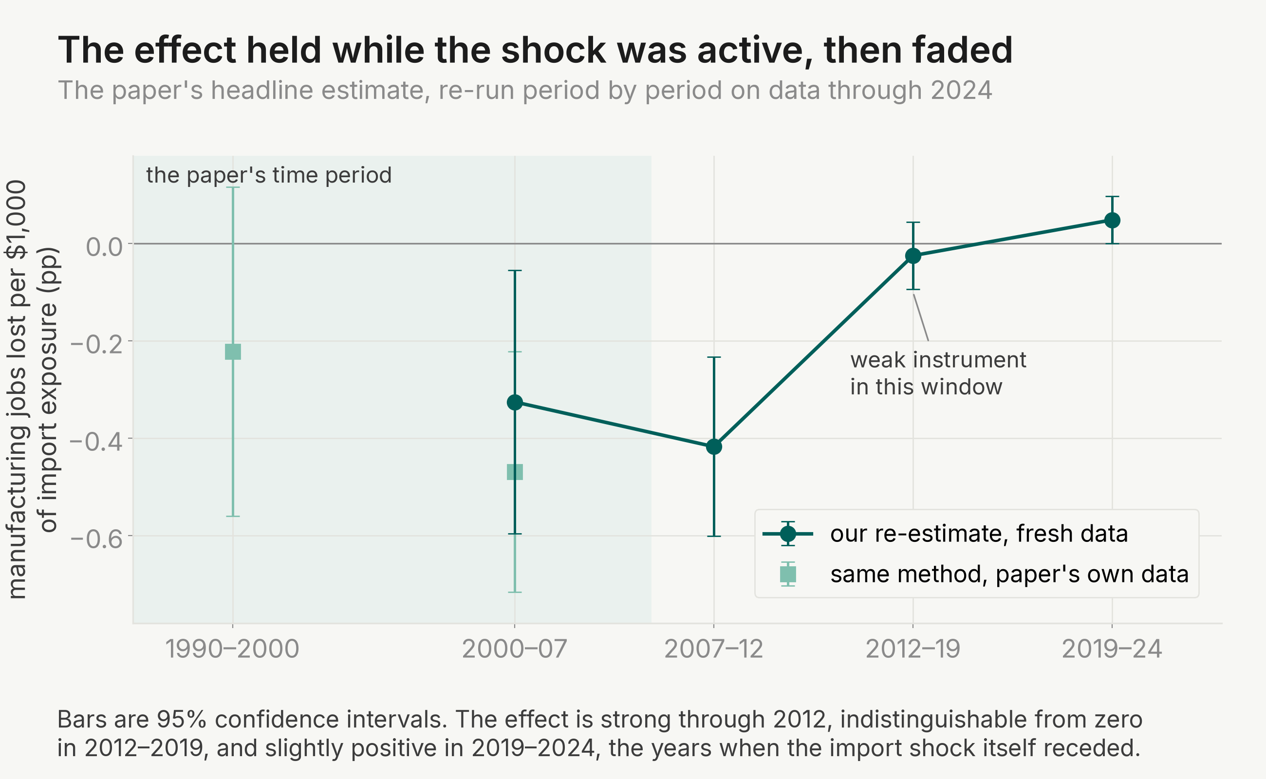
Table 3 (living). Imports from China and Local Labor Market Outcomes in CZs, 2000–2024: 2SLS Estimates
Each cell: 2SLS coefficient on (Δ imports from China to US)/worker, ten-year equivalent, column 6 controls; per $1,000 per worker.
| Outcome | ADH 1990–2007 (published) | 2000–2007 (proxy check) | 2007–2012 | 2012–2019 | 2019–2024 |
|---|---|---|---|---|---|
| Mfg emp / working-age pop (% pts) [Table 3 col 6] | −0.596*** | −0.326 | −0.417 | −0.025 | +0.048 |
| (0.099) | (0.138) | (0.094) | (0.035) | (0.025) | |
| Unemp / pop (% pts) [Table 5, panel B col 3] | +0.221*** | +0.068 | +0.005 | +0.001 | −0.002 |
| (0.058) | (0.072) | (0.125) | (0.020) | (0.021) | |
| NILF / pop (% pts) [Table 5, panel B col 4] | +0.553*** | +0.498 | −0.012 | +0.026 | −0.085 |
| (0.150) | (0.240) | (0.387) | (0.046) | (0.068) | |
| Avg log weekly wage (log pts) [Table 6, panel A col 1] | −0.759*** | −1.571 | −0.414 | −0.002 | −0.072 |
| (0.253) | (0.527) | (0.416) | (0.109) | (0.174) | |
| Log transfers per capita (log pts) [Table 8, panel A col 1] | +1.01*** | +0.729 | +0.511 | +0.020 | +0.206 |
| (0.33) | (0.337) | (0.487) | (0.069) | (0.186) | |
| Transfers per capita (2007 US$) [Table 8, panel B col 1] | +57.7 | +37.1 | +45.0 | +2.1 | +7.6 |
| (18.4) | (26.5) | (33.4) | (5.2) | (15.7) | |
| Mean ΔIPW/worker in window ($k, 10-yr equiv) | +1.14 / +1.84 per sub-period | +2.64 | +0.95 | +0.12 | −1.10 |
| First-stage F | (t = 8.9 long diff) | 29.9 | 20.8 | 6.9 † | 25.4 |
| N (commuting zones) | 1,444 (722 × 2) | 722 | 722 | 722 | 722 |
Notes: 722 mainland commuting zones per window. Outcomes 2007 onward are rebuilt from public vintages (CBP manufacturing employment / working-age population, LAUS unemployment and labor force, QCEW average weekly wage, BEA CAINC35 transfers); exposure rebuilt from CEPII BACI with the original apportionment (eq. 3) and lagged-weight instrument (eq. 4). The 2000–2007 column re-estimates the ADH window with the new data pipeline as a validation bridge. All regressions weighted by start-of-period CZ population share; standard errors clustered on state. Stars are shown only for the published column; our estimates carry standard errors, not stars. † Weak instrument in 2012–2019 (first-stage F = 6.9); the near-zero estimate there is corroborated by the reduced form and by the pooled interaction model. 2019–2024 employment weights frozen at 2011; the transfers row's last window ends 2022 (BEA vintage, N = 721).
Recalibrated on the full record, the losses read as permanent: places where import competition receded after 2019 got almost none of the jobs back.
| Parameter | Paper era (1990–2007) | Recalibrated (through 2024) |
|---|---|---|
| Impact elasticity b⁺ (mfg emp share, pp per +$1,000/worker of rising imports) | −0.596 | −0.279 (0.071) |
| Recovery rate ρ (fraction of the accumulated hit undone as imports fell) | 1.00 (full reversibility assumed) | −0.17 (the hit is permanent) |
| Net level elasticity through 2023 (pp per $1,000 accumulated) | 0 (transitory by construction) | −0.432 (0.118) |
Notes
These are the judgment calls and data limits behind our numbers, so you can decide how much weight each result deserves.
- The significance stars are the paper's, not ours: our pipeline reports coefficients and standard errors and we reprint the paper's stars alongside them.
- The extension measures jobs and wages from public series (county business data, local unemployment rates, wage records) rather than the census microdata the paper used. To show this substitution is safe, the 2000–2007 column re-runs the paper's own period on the new data; the estimates land close to the originals.
- Nothing in the paper was contradicted. The few claims that fell short of a full match are appendix results outside Table 3, and a handful of claims were not attempted or out of scope.
- Treat the 2012–2019 window with extra care: the instrument is weak there (first-stage F of 6.9), so the near-zero estimate leans on two supporting checks that agree with it.
- The last window reuses 2011 industry weights and the transfers data end in 2022, so those cells are the least current on the page. Our rebuilt trade-exposure measure tracks the paper's original at a correlation of 0.95.
The full replication working directory, including both extension studies, is public at github.com/SAI-living/living-china-syndrome.