Does Compulsory School Attendance Affect Schooling and Earnings? Angrist and Krueger (1991), replicated and extended to 2024
Angrist and Krueger asked how much an extra year of school raises your pay, apart from who stays in school. The calendar is their trick: kids born early in the year start school older and hit the legal dropout age with less schooling behind them, through no choice of their own. Across a million men in the 1970 and 1980 Censuses, the return lands at roughly 6 to 10 percent per year, close to the naive estimate.
The paper's main claims
- Men born in the first quarter finish less school, −0.124 years for the 1930–1939 cohort.
- They earn about 1.1 percent less per week, and dividing the wage gap by the schooling gap gives 0.102.
- Full TSLS agrees with OLS, so ability bias is small: 0.0891 against 0.0711.
What we got when we re-ran it
Our replication scored 0.744: 18 of the 23 extracted claims counted, 12 matched (including 2 of the 3 headline claims), 3 matched partially, 3 could not be attempted for want of data, and the other 5 were out of scope. A clean replication with a soft first stage.
Table V is the centerpiece; in each pair the paper's line comes first, ours beneath.
Table V. OLS and TSLS estimates of the return to education for men born 1930–1939: 1980 Census
| Independent variable | (1) OLS | (2) TSLS | (3) OLS | (4) TSLS | (5) OLS | (6) TSLS | (7) OLS | (8) TSLS |
|---|---|---|---|---|---|---|---|---|
| Years of education (paper) | 0.0711 (0.0003) | 0.0891 (0.0161) | 0.0711 (0.0003) | 0.0760 (0.0290) | 0.0632 (0.0003) | 0.0806 (0.0164) | 0.0632 (0.0003) | 0.0600 (0.0299) |
| Years of education (ours) | 0.0711 (0.0003) | 0.0891 (0.0161) | 0.0711 (0.0003) | 0.0760 (0.0290) | 0.0632 (0.0003) | 0.0806 (0.0164) | 0.0632 (0.0003) | 0.0600 (0.0290) |
| Race (1 = black), paper | −0.2575 (0.0040) | −0.2302 (0.0261) | −0.2575 (0.0040) | −0.2626 (0.0458) | ||||
| SMSA (1 = center city), paper | 0.1763 (0.0029) | 0.1581 (0.0174) | 0.1763 (0.0029) | 0.1797 (0.0305) | ||||
| Married (1 = married), paper | 0.2479 (0.0032) | 0.2440 (0.0049) | 0.2479 (0.0032) | 0.2486 (0.0073) | ||||
| 9 Year-of-birth dummies | Yes | Yes | Yes | Yes | Yes | Yes | Yes | Yes |
| 8 Region-of-residence dummies | No | No | No | No | Yes | Yes | Yes | Yes |
| Age, paper | −0.0772 (0.0621) | −0.0801 (0.0645) | −0.0760 (0.0604) | −0.0741 (0.0626) | ||||
| Age-squared, paper | 0.0008 (0.0007) | 0.0008 (0.0007) | 0.0008 (0.0007) | 0.0007 (0.0007) | ||||
| χ² [dof] (paper) | 25.4 [29] | 23.1 [27] | 22.5 [29] | 19.6 [27] | ||||
| χ² [dof] (ours) | 25.4 [29] | 23.1 [27] | 22.5 [29] | 19.6 [27] |
Notes. Standard errors in parentheses. Sample size is 329,509 in both the paper and our replication (the paper's Table III footnote prints 327,509 for the same men; the archive gives 329,509). Instruments are a full set of quarter-of-birth times year-of-birth interactions; each equation also includes an intercept. Our run exported the education coefficient and the overidentification statistic per column; the covariate rows (Race, SMSA, Married, Age, Age-squared) are shown from the paper alone. The one divergence anywhere in the table is the column (8) standard error, 0.0299 in the paper against 0.0290 in our run, likely a rounding or data-vintage artifact.
The first stage (Table I) is approximate by construction, run on a slightly smaller extract.
Table I. The effect of quarter of birth on various educational outcome variables (first two outcome blocks)
| Outcome variable | Birth cohort | Mean | I | II | III | F-test [P] |
|---|---|---|---|---|---|---|
| Total years of education (paper) | 1930–1939 | 12.79 | −0.124 (0.017) | −0.086 (0.017) | −0.015 (0.016) | 24.9 [0.0001] |
| Total years of education (ours) | 1930–1939 | 12.77 | −0.119 (0.017) | −0.081 (0.017) | 0.001 (0.017) | 25.1 [<0.0001] |
| Total years of education (paper) | 1940–1949 | 13.56 | −0.085 (0.012) | −0.035 (0.012) | −0.017 (0.011) | 18.6 [0.0001] |
| Total years of education (ours) | 1940–1949 | 13.57 | −0.084 (0.013) | −0.027 (0.013) | −0.019 (0.013) | 16.3 [<0.0001] |
| High school graduate (paper) | 1930–1939 | 0.77 | −0.019 (0.002) | −0.020 (0.002) | −0.004 (0.002) | 46.4 [0.0001] |
| High school graduate (ours) | 1930–1939 | 0.771 | −0.019 (0.002) | −0.019 (0.002) | −0.003 (0.002) | 44.0 [<0.0001] |
| High school graduate (paper) | 1940–1949 | 0.86 | −0.015 (0.001) | −0.012 (0.001) | −0.002 (0.001) | 54.4 [0.0001] |
| High school graduate (ours) | 1940–1949 | 0.866 | −0.014 (0.001) | −0.011 (0.001) | −0.002 (0.001) | 45.9 [<0.0001] |
Notes. Standard errors in parentheses. An MA(+2,−2) trend term was subtracted from each dependent variable; columns I, II and III are the first-, second- and third-quarter effects relative to the fourth quarter. Paper sample sizes are 312,718 (1930–1939) and 457,181 (1940–1949); ours are 294,196 and 438,507, the positive-earnings extract that shipped with the archive, so our magnitudes are approximate by construction and this exhibit was graded a partial match. The paper's further outcome blocks (postsecondary outcomes the law cannot touch) are in the original.
The companion wage tables match exactly.
Table IV. Men born 1920–1929: 1970 Census (sample size 247,199, paper and ours)
| (1) OLS | (2) TSLS | (3) OLS | (4) TSLS | (5) OLS | (6) TSLS | (7) OLS | (8) TSLS | |
|---|---|---|---|---|---|---|---|---|
| Years of education (paper) | 0.0802 (0.0004) | 0.0769 (0.0150) | 0.0802 (0.0004) | 0.1310 (0.0334) | 0.0701 (0.0004) | 0.0669 (0.0151) | 0.0701 (0.0004) | 0.1007 (0.0334) |
| Years of education (ours) | 0.0802 (0.0004) | 0.0769 (0.0150) | 0.0802 (0.0004) | 0.1310 (0.0334) | 0.0701 (0.0004) | 0.0669 (0.0151) | 0.0701 (0.0004) | 0.1007 (0.0334) |
| χ² [dof] (paper / ours) | 36.0 [29] / 36.0 [29] | 25.6 [27] / 25.6 [27] | 34.2 [29] / 34.2 [29] | 28.8 [27] / 28.8 [27] |
Table VI. Men born 1940–1949: 1980 Census (sample size 486,926, paper and ours)
| (1) OLS | (2) TSLS | (3) OLS | (4) TSLS | (5) OLS | (6) TSLS | (7) OLS | (8) TSLS | |
|---|---|---|---|---|---|---|---|---|
| Years of education (paper) | 0.0573 (0.0003) | 0.0553 (0.0138) | 0.0573 (0.0003) | 0.0948 (0.0223) | 0.0520 (0.0003) | 0.0393 (0.0145) | 0.0521 (0.0003) | 0.0779 (0.0239) |
| Years of education (ours) | 0.0573 (0.0003) | 0.0553 (0.0138) | 0.0573 (0.0003) | 0.0948 (0.0223) | 0.0520 (0.0003) | 0.0393 (0.0145) | 0.0521 (0.0003) | 0.0779 (0.0239) |
| χ² [dof] (paper / ours) | 101.6 [29] / 101.6 [29] | 49.1 [27] / 49.1 [27] | 93.6 [29] / 93.6 [29] | 50.6 [27] / 50.6 [27] |
Notes to Tables IV and VI. Standard errors in parentheses; layout and instruments as in Table V. Our replication exported the education row and the overidentification statistic per column; all match the paper's printed decimals.
The Wald estimates too, up to small standard-error differences.
Table III. Wald estimates
Panel A: 1970 Census, men born 1920–1929
| (1) Born in 1st quarter of year | (2) Born in 2nd, 3rd or 4th quarter of year | (3) Difference (std. error) (1) − (2) | |
|---|---|---|---|
| ln (wkly. wage), paper | 5.1484 | 5.1574 | −0.00898 (0.00301) |
| ln (wkly. wage), ours | 5.1485 | 5.1574 | −0.00898 (0.00302) |
| Education, paper | 11.3996 | 11.5252 | −0.1256 (0.0155) |
| Education, ours | 11.3996 | 11.5252 | −0.1256 (0.0156) |
| Wald est. of return to education (paper / ours) | 0.0715 (0.0219) / 0.0715 (0.0241) | ||
| OLS return to education (paper / ours) | 0.0801 (0.0004) / 0.0801 (0.0004) |
Panel B: 1980 Census, men born 1930–1939
| (1) Born in 1st quarter of year | (2) Born in 2nd, 3rd or 4th quarter of year | (3) Difference (std. error) (1) − (2) | |
|---|---|---|---|
| ln (wkly. wage), paper | 5.8916 | 5.9027 | −0.01110 (0.00274) |
| ln (wkly. wage), ours | 5.8916 | 5.9027 | −0.01110 (0.00274) |
| Education, paper | 12.6881 | 12.7969 | −0.1088 (0.0132) |
| Education, ours | 12.6881 | 12.7969 | −0.1088 (0.0133) |
| Wald est. of return to education (paper / ours) | 0.1020 (0.0239) / 0.1020 (0.0252) | ||
| OLS return to education (paper / ours) | 0.0709 (0.0003) / 0.0709 (0.0003) |
Notes. The Wald estimate is the first-quarter wage gap divided by the first-quarter education gap. Point estimates match the paper at all printed decimals; the Wald standard errors differ slightly (0.0219 against 0.0241 in Panel A, 0.0239 against 0.0252 in Panel B), most likely a delta-method implementation detail.
The same analysis on today's data
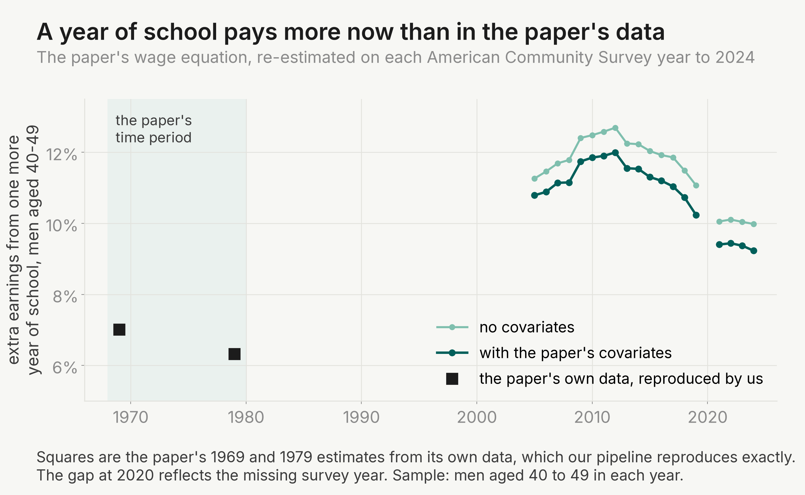
The experiment can't be rerun: quarter of birth left the public microdata after 1980, and with 97.2 percent of sixteen-year-olds now enrolled the laws no longer bind. So we held the paper's age window, men 40 to 49, and re-ran its OLS wage equation on every American Community Survey year, 2005 to 2024; the return climbed from 0.063 in 1979 to near 0.12 around 2010–2013, easing to 0.092 by 2024. The equation is the paper's
with the weekly wage, years of education, year-of-birth dummies and the return; TSLS instruments with the 30 quarter-times-year-of-birth interactions.
Table V, continued. OLS estimates of the return to education for men aged 40-49: American Community Survey, 2005–2024
| Independent variable | 2005 | 2010 | 2015 | 2019 | 2021 | 2024 |
|---|---|---|---|---|---|---|
| Years of education, no covariates | 0.1126 (0.0009) | 0.1248 (0.0009) | 0.1204 (0.0009) | 0.1107 (0.0010) | 0.1005 (0.0010) | 0.0998 (0.0010) |
| Years of education, with covariates | 0.1079 (0.0009) | 0.1185 (0.0008) | 0.1130 (0.0009) | 0.1024 (0.0009) | 0.0940 (0.0010) | 0.0923 (0.0009) |
| Age dummies | Yes | Yes | Yes | Yes | Yes | Yes |
| Sample size | 181,686 | 168,179 | 154,144 | 153,525 | 149,845 | 162,478 |
Notes. Standard errors in parentheses. The first row mirrors the paper's column (1) specification (age controls only); the second mirrors column (5), adding race, marital status and region dummies. As a continuity check, the same pipeline on the paper's own archive data returns its column (5) values exactly: 0.0701 for 1969 earnings and 0.0632 for 1979. ACS education is categorical attainment mapped to years, so the return is per mapped year; the ACS has no SMSA variable, and dropping SMSA on the 1980 archive data moves the column (5) coefficient by only +0.0026. There is no 2020 ACS one-year file.
We also ran modern weak-instrument diagnostics on the original samples.
Modern weak-instrument inference on the original samples (column (5)-(6) specification)
| Sample | OLS | TSLS | LIML | First-stage F | Anderson-Rubin 95% set |
|---|---|---|---|---|---|
| Men born 1920–1929: 1970 Census | 0.0701 (0.0004) | 0.0669 (0.0151) | 0.0658 (0.0174) | 4.55 | [0.010, 0.122] |
| Men born 1930–1939: 1980 Census | 0.0632 (0.0004) | 0.0806 (0.0164) | 0.0838 (0.0179) | 4.75 | [−0.002, 0.178] |
| Men born 1940–1949: 1980 Census | 0.0520 (0.0003) | 0.0393 (0.0145) | 0.0286 (0.0197) | 6.85 | empty (over-identification rejected) |
Notes. Standard errors in parentheses. Instruments are the paper's 30 quarter-of-birth times year-of-birth interactions. A first-stage F between 4.6 and 6.9 is weak by any modern rule of thumb, the Anderson-Rubin confidence sets are wide where they exist, and for the 1940–1949 sample the set is empty because the overidentifying restrictions are rejected at every candidate value of the return.
The first-quarter schooling deficit was already fading: −0.167 for men born 1920–1929, −0.119 for 1930–1939, −0.084 for 1940–1949.
Notes
These are the judgment calls and data limits behind our numbers, so you can decide how much weight each result deserves.
- Our Table I uses the positive-earnings extract (294,196 and 438,507 men), smaller than the paper's samples (312,718 and 457,181); hence the partial grade.
- Point estimates match the printed decimals throughout Tables III–VI; the gaps are standard errors: Table V column (8) (0.0299 vs 0.0290) and the Table III Wald rows.
- Table II's enrollment difference-in-differences had no archived data; Tables VII and VIII, the log-weeks variant and the footnote checks were out of scope by design.
- ACS education is categorical attainment mapped to years, with no SMSA control (worth +0.0026 on the 1980 data) and no 2020 one-year file.
The full replication working directory, including both extension studies, is public at github.com/SAI-living/living-compulsory-schooling.