Reassessing the Ins and Outs of Unemployment: Shimer (2012), replicated and extended to 2026
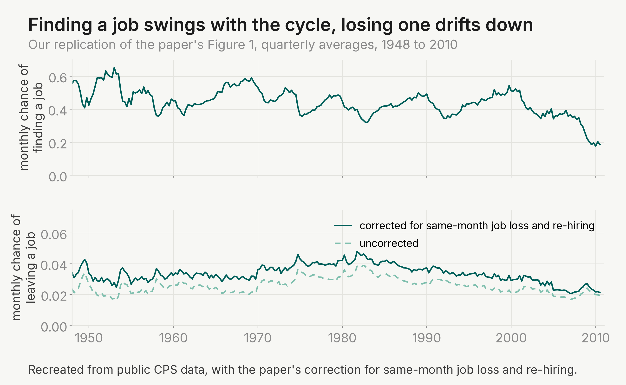
Shimer (2012) asks whether recessions raise unemployment because more workers lose their jobs or because the unemployed take longer to find new ones. From public CPS data for 1948–2010 he builds monthly job finding and job loss probabilities and asks which one drives the unemployment rate. The answer is slower hiring: 0.77 of the fluctuations over the full sample, and 0.90 since 1987.
The paper's main claims
- Slower job finding explains most unemployment fluctuations over 1948–2010: 0.77.
- Since 1987 it explains almost everything: 0.90.
- Job loss explains a quarter or less: 0.24.
- Adding labour force entry and exit, job finding still leads since 1987: 0.51.
What we got when we re-ran it
We graded 27 extracted claims, 25 counted: 13 matched, 5 partial (C2, C4, C15, C17, C19), 1 not matched, 6 not attempted for want of undeposited microdata, and 2 (C20, C26) out of scope. The score is 0.63: solid on the core result, rough at the input edges.
| (1) | (2) | (3) | (4) | (5) | |
|---|---|---|---|---|---|
| all workers | all workers | all workers | all workers | men 25-54 | |
| 1948–2010 | 1967–2010 | 1976–2010 | 1987–2010 | 1976–2010 | |
| x̄/(x̄ + fₜ), published | 0.77 | 0.83 | 0.85 | 0.90 | 0.69 |
| x̄/(x̄ + fₜ), this replication | 0.763 | 0.807 | 0.838 | 0.858 | n.a. |
| xₜ/(xₜ + f̄), published | 0.24 | 0.17 | 0.15 | 0.10 | 0.32 |
| xₜ/(xₜ + f̄), this replication | 0.245 | 0.198 | 0.166 | 0.144 | n.a. |
Table 1: Decomposition: job finding and employment exit rates. Notes: the first row is the coefficient from a regression of the detrended hypothetical rate x̄/(x̄ + fₜ) on the detrended actual rate uₜ₊₁/lₜ₊₁, the second the same for xₜ/(xₜ + f̄); all series are quarterly averages of monthly data, HP detrended with smoothing parameter 10⁵. The paper reports no standard errors and neither do we here. Roman rows are the paper's published values; italic rows are our replicated values. Column 5 requires matched CPS microdata for prime age men and was out of the replication's scope. Our short term unemployment series splices shipped microdata shares onto published levels after 2005, a documented and conservative departure from the shipped code.
| (1) | (2) | (3) | (4) | |
|---|---|---|---|---|
| unemployment rate | unemployment rate | employment-population ratio | employment-population ratio | |
| published period | 1967–2010 | 1987–2010 | 1967–2010 | 1987–2010 |
| replicated period | 1967–2004 | 1987–2004 | 1967–2004 | 1987–2004 |
| λᴱᵁ | 0.22 / 0.218 | 0.17 / 0.134 | 0.37 / 0.420 | 0.30 / 0.281 |
| λᴱᴵ | −0.05 / -0.044 | −0.05 / -0.036 | −0.36 / -0.313 | −0.40 / -0.262 |
| λᵁᴱ | 0.49 / 0.504 | 0.51 / 0.553 | 1.05 / 1.040 | 1.16 / 1.182 |
| λᵁᴵ | 0.17 / 0.181 | 0.16 / 0.176 | −0.48 / -0.521 | −0.50 / -0.545 |
| λᴵᴱ | 0.08 / 0.072 | 0.09 / 0.075 | 0.69 / 0.644 | 0.73 / 0.679 |
| λᴵᵁ | 0.12 / 0.095 | 0.13 / 0.098 | −0.36 / -0.278 | −0.42 / -0.315 |
Table 2: Decomposition: entry and exit from the labour force. Notes: each cell shows the paper's published value, then our replicated value in italics; each is the coefficient from a regression of the detrended hypothetical rate, letting only the named transition rate vary, on the detrended actual rate, on quarterly averages HP detrended with smoothing parameter 10⁵. Replicated columns end in 2004Q4 because the shipped transition rate files stop there, which concentrates the deviations in the 1987 columns (claim C17 graded partial).
The same analysis on today's data
We rebuilt both series from live BLS and CPS data through June 2026; on the paper's own windows our pipeline matches to within 0.01. Without 2020, the 1987–2026 job finding share is 0.892 against the paper's 0.90. With 2020 in, the 2010–2026 exit share hits 0.380: the pandemic was a layoff shock, and for once the ins won.
The core object is
the chance of finding a job in month ; is the number unemployed, the number unemployed under five weeks. The exit probability comes from the flow equation, and each table row regresses a detrended hypothetical rate, one rate moving at a time, on the detrended actual rate.
Panel A: excluding 2020 (headline)
| (1) | (2) | (3) | (4) | |
|---|---|---|---|---|
| all workers | all workers | all workers | all workers | |
| 1948–2026 | 1967–2026 | 1976–2026 | 1987–2026 | |
| x̄/(x̄ + fₜ) | 0.791 (0.025) | 0.846 (0.023) | 0.859 (0.024) | 0.892 (0.021) |
| xₜ/(xₜ + f̄) | 0.209 (0.030) | 0.147 (0.031) | 0.131 (0.032) | 0.101 (0.030) |
Panel B: including 2020
| 1948–2026 | 1967–2026 | 1976–2026 | 1987–2026 | 2010–2026 | |
|---|---|---|---|---|---|
| x̄/(x̄ + fₜ) | 0.738 (0.050) | 0.754 (0.077) | 0.754 (0.086) | 0.762 (0.102) | 0.538 (0.103) |
| xₜ/(xₜ + f̄) | 0.250 (0.043) | 0.221 (0.066) | 0.217 (0.073) | 0.208 (0.086) | 0.380 (0.101) |
Table 3: The paper's Table 1 decomposition on samples extended to 2026Q2. Notes: same construction as Table 1, all workers, quarterly averages HP detrended with smoothing parameter 10⁵; Newey-West standard errors with 8 lags in parentheses are ours, the paper reports none. Panel A drops 2020Q1-2020Q4; Panel B keeps them, with the March 2020 exit spike clipped as described in the fine print.
The three state version anchors on 1990–2010, within 0.02 of the paper throughout.
| published, 1987–2010 | this study, 1990–2010 | 1990–2026, excluding 2020 | 2010–2026, including 2020 | |
|---|---|---|---|---|
| λᴱᵁ | 0.17 | 0.168 (0.022) | 0.167 (0.022) | 0.551 (0.140) |
| λᴱᴵ | −0.05 | −0.034 (0.006) | −0.043 (0.006) | −0.025 (0.013) |
| λᵁᴱ | 0.51 | 0.520 (0.022) | 0.488 (0.018) | 0.150 (0.097) |
| λᵁᴵ | 0.16 | 0.152 (0.015) | 0.139 (0.011) | 0.094 (0.020) |
| λᴵᴱ | 0.09 | 0.079 (0.009) | 0.087 (0.006) | 0.064 (0.012) |
| λᴵᵁ | 0.13 | 0.115 (0.016) | 0.154 (0.012) | 0.195 (0.006) |
Table 4: The paper's Table 2 decomposition, unemployment rate columns, extended to 2026Q2. Notes: same construction as Table 2; Newey-West standard errors with 8 lags in parentheses are ours, the paper reports none. Flows are built from live BLS gross flows series with the paper's eigenvalue time aggregation correction; every month passed the real, positive, distinct eigenvalue check; the flows are not adjusted for margin error, and the employment-population columns cannot be extended from published flows alone.
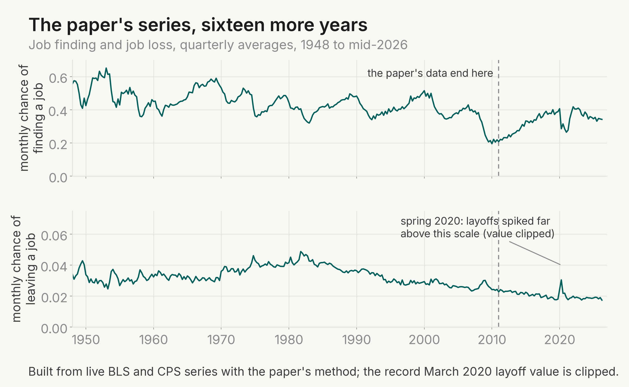
Both flows also fell in level; the market converges more slowly now.
| parameter | 1948–2010 | 2010–2026 |
|---|---|---|
| mean employment exit probability X̄ | 0.033 | 0.021 |
| adjustment speed ω = F̄ + X̄ | 0.473 | 0.342 |
| half-life of an unemployment deviation (months) | 1.08 | 1.66 |
| implied steady state unemployment u* | 0.071 | 0.062 |
| separation share of the 2020 unemployment surge | n.a. | 0.81 |
Notes
These are the judgment calls and data limits behind our numbers, so you can decide how much weight each result deserves.
- Table 1 column 5 and six claims (C12, C21–C25) need undeposited CPS microdata; the one non-match (C11) is the paper's Figure 2.
- The shipped transition rate files stop in 2004Q4, so our Table 2 columns end there (C17 partial).
- The weakest cell, the 1987–2010 exit share (0.144 vs 0.10, C2 partial), is a short term unemployment vintage issue; the extension adjusts the 1994 CPS redesign differently from the replication and gets 0.107.
- The three state extension covers only the unemployment rate half of Table 2; published BLS flows begin in February 1990 and are not margin-adjusted.
- Newey-West standard errors (8 lags) are ours; the paper reports none.
- March 2020's exit spike is clipped, 2020 windows are shown with and without 2020Q1–2020Q4, and the late 2025 shutdown gap is dropped, never interpolated.
The full replication working directory, including both extension studies, is public at github.com/SAI-living/living-ins-and-outs.