Regional Evolutions: Blanchard and Katz (1992), reconstructed and extended to 2025
Blanchard and Katz asked whether a state that loses jobs gets them back or loses workers instead. They took annual state data for 1947–90, all relative to the US average, and traced shock responses with autoregressions and a VAR. The jobs never come back: employment settles 1.3 percent below its old path, while unemployment and participation recover in five to seven years as people move away.
The paper's main claims
- Relative employment shocks are permanent: a 1 percent loss ends 1.3 percent down for good.
- Year one: unemployment up 0.32 points, participation down 0.17.
- Both vanish within 5–7 years.
- Out-migration absorbs 0.65 of each lost job in year one.
- State growth persists: 1970–90 on 1950–70 has slope 0.70.
What we got when we re-ran it
No replication package survives; we rebuilt the panel from public BLS and BEA data. Our verifier scored 32 of the 35 extracted claims: a strict replication score of 0.296, the seven headline claims splitting 1 match, 4 partial, 2 no match. Low, with a clean pattern: employment reproduces closely, the wage and early-unemployment exhibits only partly.
Table 1 side by side.
Table 1. Univariate Models of Relative Employment, Unemployment, and Wages
| Result | Log employment change (paper) | (ours) | Unemployment rate (paper) | (ours) | Log wage (paper) | (ours, per-capita income proxy) |
|---|---|---|---|---|---|---|
| Regression results | ||||||
| Coefficient on lagged dependent variable | ||||||
| One lag | 0.492 (0.023) | 0.516 (0.022) | 0.899 (0.032) | 1.075 (0.037) | 1.072 (0.023) | 0.818 (0.022) |
| Two lags | −0.099 (0.025) | −0.129 (0.025) | −0.159 (0.033) | −0.355 (0.034) | −0.129 (0.034) | 0.078 (0.028) |
| Three lags | 0.010 (0.024) | 0.027 (0.024) | n.a. | n.a. | 0.057 (0.034) | 0.038 (0.027) |
| Four lags | −0.054 (0.022) | −0.066 (0.022) | n.a. | n.a. | −0.074 (0.024) | −0.049 (0.020) |
| Standard error | 0.017 | n.a. | 0.083 | n.a. | 0.016 | n.a. |
| Implied impulse responses | ||||||
| Year 1 | 1.00 | 1.00 | 1.00 | 1.00 | 1.00 | 1.00 |
| Year 2 | 1.49 | 1.52 | 0.90 | 1.07 | 1.07 | 0.82 |
| Year 3 | 1.63 | 1.65 | 0.65 | 0.80 | 1.02 | 0.75 |
| Year 4 | 1.67 | 1.68 | 0.44 | 0.48 | 1.01 | 0.71 |
| Year 5 | 1.62 | 1.63 | 0.29 | 0.23 | 0.94 | 0.63 |
| Year 10 | 1.52 | 1.53 | 0.04 | −0.02 | 0.57 | 0.30 |
| Year 20 | 1.53 | 1.53 | 0.01 | n.a. | 0.19 | 0.09 |
Notes: Paper columns are the published values. Source (paper): estimates of univariate equations using data described in the paper's appendix; periods of estimation are 1952–90 for employment and wages and 1972–90 for unemployment; standard errors of the coefficients are in parentheses. Our columns: employment 1952–90 from FRED/BLS reconstructions (n = 1,953); unemployment 1976–90 LAUS only (n = 663), against the paper's 1972–90 panel with constructed pre-1976 data; wage proxied by per-capita income (n = 1,985). Replicated impulse responses are re-indexed to the paper's convention with Year 1 = 1.00 at impact. The regression standard error row and the unemployment Year 20 cell were not stored by our run (n.a.).
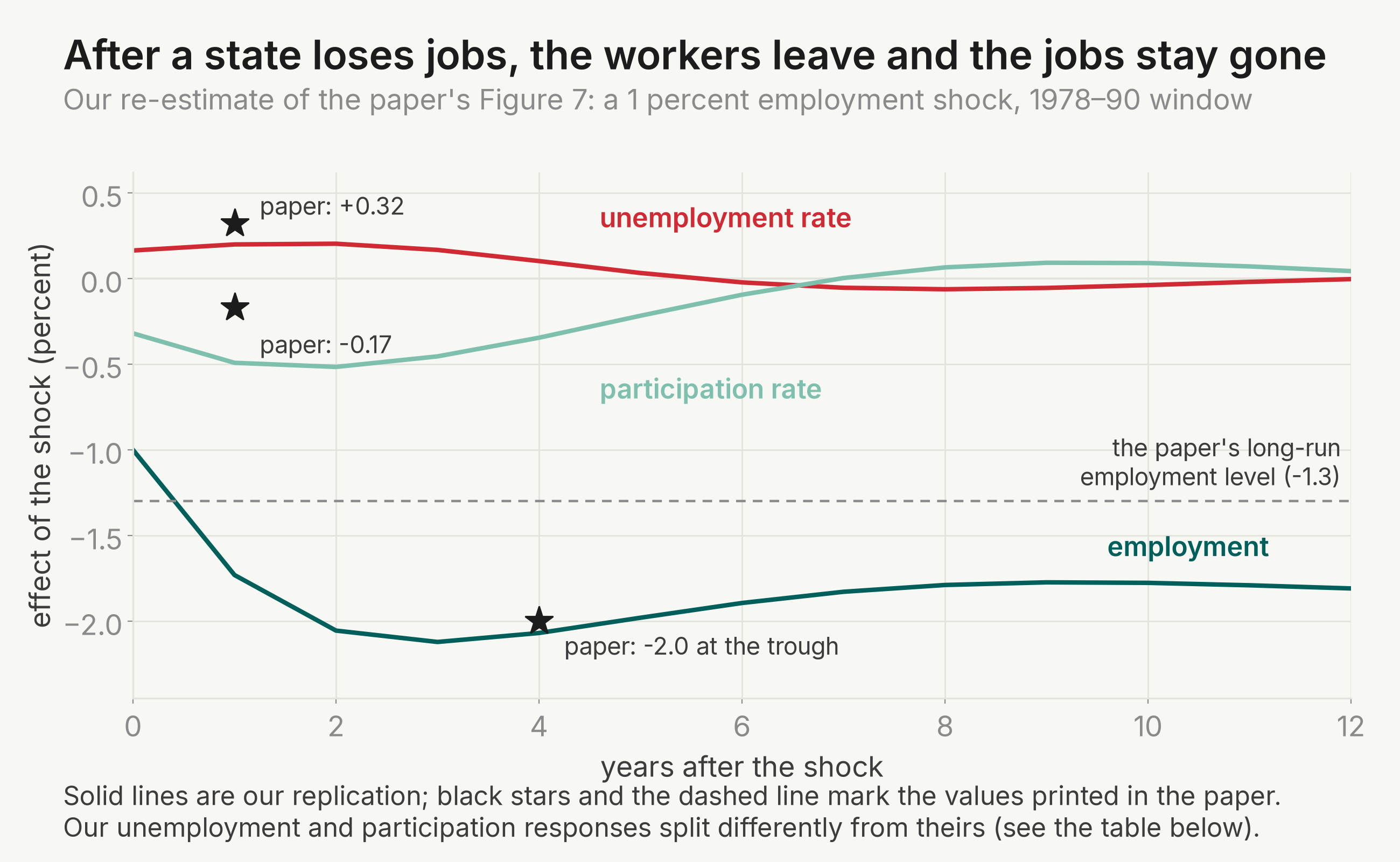
Our version of Figure 7.
| Quantity (paper's text, pp. 33-34) | Paper | Ours |
|---|---|---|
| Year-1 rise in unemployment rate (pp) | 0.32 | 0.20 |
| Year-1 fall in participation rate (pp) | 0.17 | 0.49 |
| Peak employment response (percent, ~year 4) | −2.0 | −2.1 |
| Employment plateau (percent) | −1.3 | −1.8 |
| Years until unemployment and participation effects disappear | 5-7 | 11 (U), 7 (P) |
| Per-worker split of a 1-job loss, year 1: unemployment | 0.3 | 0.12 |
| ... participation | 0.05 | 0.28 |
| ... implied net out-migration | 0.65 | 0.60 |
Notes: paper values are the published text quantities; ours are from the trivariate VAR re-estimated on 1978–90 with LAUS/CPS-derived series and resident population proxying working-age population. The split of the first-year adjustment between unemployment and participation does not replicate on our household-basis series, though the implied net out-migration share (0.60 against 0.65) and the employment path (peak, hump shape, permanence) do; the paper's own footnote 37 reports that the household basis gives a smaller initial migration share (0.40) than its establishment-basis headline (0.65).
And the opening scatter.
| Quantity | Paper | Ours |
|---|---|---|
| Regression slope | 0.70 | 0.698 |
| R² | 0.75 | 0.754 |
| R² excluding AZ, FL, NV | 0.60 | 0.61 |
The same analysis on today's data
We rolled the panel forward to 2025 and re-ran everything window by window (only 1978–90 is the paper's own; brackets are 90 percent bootstrap bands). Permanence survives the Great Recession and COVID, but migration absorbs less of a first-year loss (0.24–0.28 after 2008 vs 0.38 then) and growth persistence has halved. The quantities come from the paper's trivariate VAR:
with relative employment growth, , the relative log employment and participation rates, and shock ordered first.
Permanence first.
| Result | Log employment change, 1952–90 (paper) | 2006–25 (ours) | Unemployment rate, 1972–90 (paper) | 2011–25 (ours) | Log wage |
|---|---|---|---|---|---|
| Year 4 | 1.67 | 1.62 [1.37, 1.89] | 0.44 | not computed | not extended |
| Year 5 | 1.62 | not computed | 0.29 | 0.08 [0.05, 0.11] | not extended |
| Year 10 | 1.52 | not computed | 0.04 | 0.01 [0.00, 0.01] | not extended |
| Year 20 | 1.53 | 1.52 [1.30, 1.78] | 0.01 | ~0 (implied) | not extended |
Notes: paper columns are the published Table 1 impulse responses; ours re-estimate the same pooled autoregressions on the modern windows shown, with 90 percent state-cluster bootstrap bands in brackets. The sweep stored only the horizons shown; the wage column is not extendable because no modern equivalent of the paper's manufacturing production-worker earnings series exists.
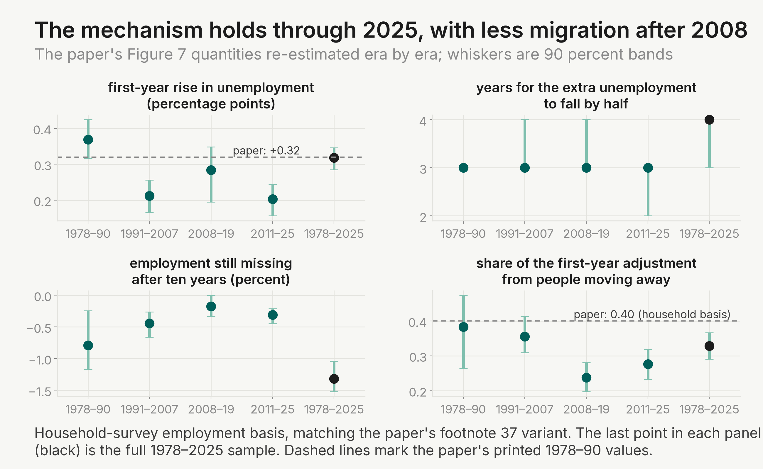
The Figure 7 quantities era by era.
| Quantity | 1978–90 (paper's window) | 1991–2007 | 2008–19 | 2011–25 | Full 1978–2025 |
|---|---|---|---|---|---|
| Year-1 rise in unemployment rate (pp) | 0.37 [0.32, 0.42] | 0.21 [0.17, 0.26] | 0.28 [0.19, 0.35] | 0.20 [0.16, 0.24] | 0.32 [0.28, 0.35] |
| UR half-life (years) | 3 [3, 3] | 3 [3, 4] | 3 [3, 4] | 3 [2, 3] | 4 [3, 4] |
| Year-10 employment response (percent) | −0.79 [−1.17, −0.25] | −0.45 [−0.66, −0.26] | −0.17 [−0.33, −0.00] | −0.31 [−0.45, −0.21] | −1.32 [−1.52, −1.04] |
| Year-1 out-migration share of adjustment | 0.38 [0.26, 0.47] | 0.36 [0.31, 0.41] | 0.24 [0.20, 0.28] | 0.28 [0.23, 0.32] | 0.33 [0.29, 0.37] |
Notes: household employment basis, 90 percent state-cluster bootstrap bands in brackets; window labels follow the paper's sample notation but, except for 1978–90, are our era choices. Anchor: the paper's printed 1978–90 values (establishment basis) are a +0.32 point first-year unemployment rise, effects gone in five to seven years, a −1.3 percent employment plateau, and a 0.65 first-year migration share (0.40 on the household basis of its footnote 37, the basis our panel uses). The full-sample first-year unemployment response of 0.32 landing on the printed +0.32 is a coincidence of the pooled sample, not a replication.
On the payroll basis the migration share falls 0.77 to 0.63, and the model refits with a halved migration parameter.
And the scatter, pair by pair.
| Sample pair | Slope | 90% CI | R² |
|---|---|---|---|
| 1970–90 on 1950–70 (paper) | 0.70 | n.a. | 0.75 |
| 1970–90 on 1950–70 (ours) | 0.71 | [0.62, 0.81] | 0.76 |
| 1990–2007 on 1970–90 | 0.64 | [0.54, 0.75] | 0.67 |
| 2007–25 on 1990–2007 | 0.37 | [0.28, 0.47] | 0.46 |
Notes
These are the judgment calls and data limits behind our numbers, so you can decide how much weight each result deserves.
- Table 1's wage column is a per-capita-income proxy (the paper's manufacturing wage series is gone); the published overshoot (1.07 at year 2) comes out 0.82.
- The paper's unemployment sample is 1972–90 with constructed pre-1976 data, ours LAUS-only 1976–90 (n = 663), hence our faster decay (0.23 vs 0.44 at year 4; the paper prints 0.29 at year 5).
- Our household-basis series miss the year-1 split (+0.20 vs +0.32, −0.49 vs −0.17) and deepen the plateau (−1.8 vs −1.3; payroll recovers −1.5); footnote 37 reports the same gap (0.40 vs 0.65).
- Unstored cells (the standard error row, unemployment Year 20, some extension horizons) show n.a., never interpolations; impulse responses are re-indexed to Year 1 = 1.00.
- Okun coefficients and state-level long-run responses are left off (non-comparable units; near-unit-root explosions); everything here is pooled.
- All windows except 1978–90 are our era choices.
The full replication working directory, including both extension studies, is public at github.com/SAI-living/living-regional-evolutions.